Leaking Data Through 5 Volts: The USB Power Line as a Covert Channel
Ever noticed how many signal forensics challenges in CTFs an AI can break in seconds? I made one that held out against AI for almost 7 hours.
It’s called TX, an old forensics challenge of mine from GCUP 2.0 CTF, organized by Securinets in collaboration with the Institut français de Tunisie (IFT). It was finally solved with Codex. The flag leaks through the one part of a USB port nobody watches: the power line.
Every USB port gives a device two things: a data connection and 5 volts. Security people spend almost all their attention on the first one. We block mass storage, allowlist keyboards, and hand out “charge-only” cables and data blockers. The power pins get ignored, because power isn’t data.
It can be. The voltage on a power line depends on how much current every device on it draws, and anything that shares the line can measure that voltage. So a device that controls its current can send, and a device that watches its supply voltage can receive, with no data connection between them.
This post starts with that phenomenon: why power lines leak, what published research has done with it, and why the usual USB defenses miss it. Then it goes into how TX was built and how to solve it.
Part 1: The phenomenon
Power has been leaking secrets for a long time
Using power as a leak isn’t new. In 1999, Kocher, Jaffe and Jun published Differential Power Analysis: record a smart card’s power consumption over many runs of a cryptographic algorithm, and statistics on those traces recover its secret key. The chip isn’t doing anything wrong. Transistors draw current when they switch, what switches depends on the data, so the data ends up in the current.
Two terms help here:
- A side channel is an unintentional leak. The device isn’t trying to send anything, and the attacker listens to a by-product: power, timing, EM radiation, sound.
- A covert channel is intentional. Something already compromised wants to get data out, and hides it in a medium nobody is watching.
TX is the second kind: a malicious device that modulates the power line on purpose.
Why a USB port’s voltage moves
A USB port isn’t a perfect 5 V source. Between the regulator and your device there is always some resistance: the regulator’s own output impedance, the current-limit switch or polyfuse that protects the port, PCB traces, connector contacts, the cable. When the current changes, the voltage changes with it, by Ohm’s law: ΔV = ΔI · R.
The numbers are small but measurable. A few hundred milliohms of resistance and a 100 mA change in current gives tens of millivolts. Fast changes also hit the regulator, which can’t react instantly. Its output capacitors cover the gap, the voltage dips, then the control loop pulls it back, often overshooting a bit. So a burst of current shows up on the rail as a short, smooth pulse, not a clean step.
In TX’s story, the extra electronics inside the keyboard are a capacitor bank. It charges slowly, then dumps charge in short bursts back onto VBUS, so the voltage briefly goes up. A normal keyboard never pushes current back into the host’s VBUS, and that’s part of what makes this one malicious.
A shared rail is a party line
Every device on the same hub hangs off the same VBUS node. The resistance they share (the hub’s regulator, its switch, its traces) is what couples them. When one device changes its current, the voltage at that shared node moves, and every other device on the node can measure it.
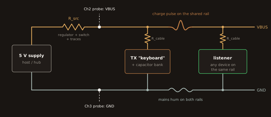
One rail, many listeners: the transmitter and the listener only share power, never data
The listener doesn’t need a data connection to the transmitter, a driver, or any permission on the host. It needs an ADC on its own power input.
This has been shown in published research:
- USB Snooping Made Easy (Su, Genkin, Ranasinghe, Yarom, USENIX Security 2017). The authors tested over 50 computers and external hubs, and more than 90% leaked USB traffic to other ports on the same hub through crosstalk. The leak is visible on the power lines too, which defeats charge-only cables. They demonstrated it with a modified novelty USB lamp that captured and exfiltrated traffic from other devices on the hub, like keyboards, card readers and fingerprint readers.
- Charger-Surfing (Cronin, Gao, Yang, Wang, USENIX Security 2021). A smartphone’s power draw through its USB charging cable leaks what’s happening on its screen. It leaks enough to infer button presses and to crack a 4-digit passcode on the first try about 95% of the time.
- PowerHammer (Guri, Zadov, Bykhovsky, Elovici, 2018). Malware on an air-gapped computer modulates CPU load, which modulates the current the machine draws from the mains. The data is received by tapping the building’s power lines, either near the outlet or at the electrical panel.
TX is the same idea at USB scale: a covert transmitter on VBUS instead of a PC on the mains.
Why the usual USB defenses don’t see it
- Data blockers and charge-only cables cut D+ and D−. They have to pass VBUS and GND, or the device gets no power. VBUS and GND are exactly where this channel lives.
- USB device policies (like USBGuard on Linux) decide based on what the device says it is. This one is a real keyboard with real HID reports. Even when a policy blocks a device, the port usually keeps powering it, and power is all the transmitter needs.
- USB power meters, the little inline gadgets, update a few times per second and show averages. One-millisecond, 30 mV pulses vanish in the average. The modulation makes this worse (see below): every time slot has exactly one pulse, so the average current doesn’t depend on the data at all.
What does help: physical control over what gets plugged into sensitive machines, not sharing a power rail between trusted and untrusted devices, and, if a device looks suspicious, looking at VBUS with an oscilloscope instead of a USB meter.
What a real power rail looks like
A clean 5 V line doesn’t exist. On a real rail you typically find:
- Mains hum: 50 Hz here in Tunisia (60 Hz in the Americas), coupled in through ground loops between the PC, the analyzer and the wall. It shows up on GND too, which matters later.
- USB bus activity: full-speed USB sends a Start-of-Frame packet every 1 ms, so there’s often a 1 kHz rhythm in the current draw.
- Switching-regulator ripple: usually hundreds of kHz or more, too fast for a 10 kS/s channel to see.
- Plain noise from the ADC and everything around it.
At TX’s time scale, two of these matter: 50 Hz hum on both VBUS and GND, and random noise. The pulses are about the same size as the noise, and the whole challenge comes from that.
Part 2: The challenge
The scenario
A suspicious USB device was found plugged into a secure workstation. Externally it looked like a standard keyboard, but it contained extra electronics including a large capacitor bank. Your task: recover the data that was exfiltrated via a clever side-channel.
Players got two files:
capture.sal: a Saleae Logic 2 capture with 4 unlabeled channels (2 digital @ 1 MS/s, 2 analog @ 10 kS/s)usb_traffic.pcap: USB traffic from a “USB analyser”
Designing the transmitter
The signal has three layers, from the voltage up to the flag.
Layer 1: pulse-position modulation (PPM). Time is split into 10 ms slots, and every slot gets exactly one pulse. The information is where the pulse sits inside the slot:
- pulse centred at 2 ms, symbol 0
- pulse centred at 7 ms, symbol 1
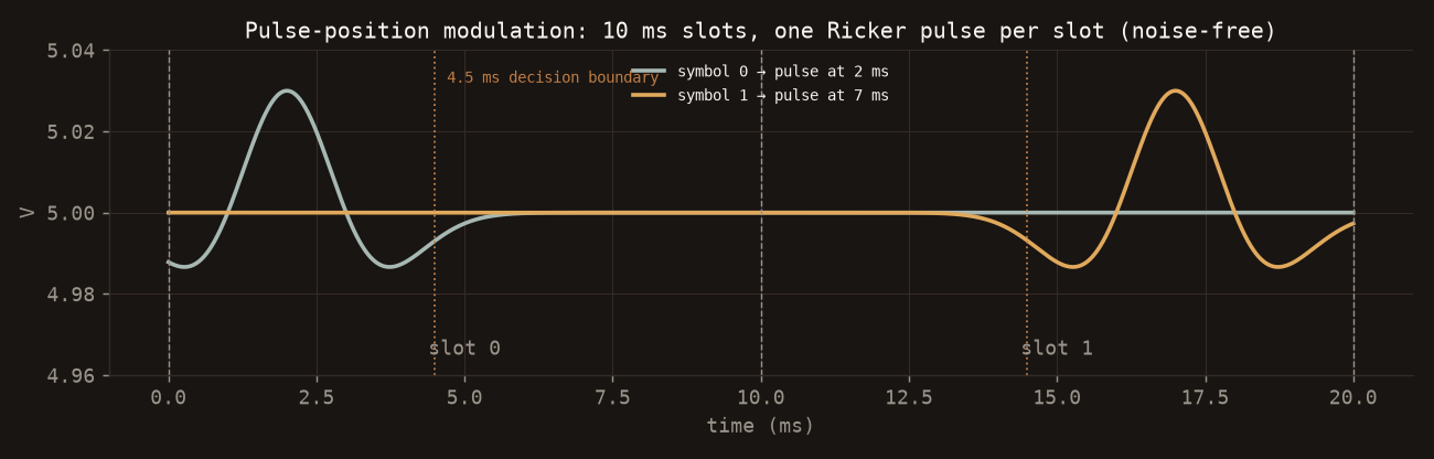
One symbol per 10 ms slot. The pulse is a Ricker wavelet (τ = 1 ms, 30 mV)
The pulse shape is a Ricker wavelet (the “Mexican hat”): a smooth bump with a small undershoot on each side and zero net area. It’s a standard model pulse in seismology, and it’s close to what a short burst looks like on a rail where decoupling capacitors smooth the edges and a regulator pulls the voltage back.
def ricker_pulse(t, t_centre):
    dt = (t - t_centre) / PULSE_TAU          # PULSE_TAU = 1 ms
    return PULSE_DROP * (1 - dt*dt) * math.exp(-dt*dt / 2)   # PULSE_DROP = 30 mV
PPM suits a covert transmitter well:
- The average power doesn’t depend on the data. One pulse per slot, always, so the capacitor bank discharges at a fixed rate and a power meter sees a steady load.
- The receiver gets timing for free, because pulses arrive every 10 ms no matter what.
- The transmitter is simple. It needs one timer and one decision: fire early or fire late.
Layer 2: Manchester. Each data bit becomes two PPM symbols:
| bit | symbols |
|---|---|
| 0 | 1 0 |
| 1 | 0 1 |
Manchester guarantees a transition in every bit, and it gives a free sanity check: a pair like 00 or 11 means a symbol was read wrong.
Layer 3: the frame.
[ 64-bit preamble 1010… ][ sync 0xEB 0x90 ][ flag bytes ][ CRC-8/MAXIM ]
The preamble gives a clean alternating pattern to lock onto, 0xEB90 is a classic telemetry sync word, and the CRC tells you whether your decode is actually right.
That’s 64 + 16 + 39·8 + 8 = 400 bits, so 800 symbols, so 8 seconds of transmission in a 10-second capture.
The rabbit holes (on purpose)
Two of the three data sources are there to waste your time.
The pcap. It’s a HID keyboard capture. Decode the key reports and you get:
the quick brown fox jumps over the lazy dog
all your base are belong to us
No flag. The keyboard really is a keyboard. There’s one useful detail: the host polls it every 10 ms, the same length as a PPM slot.
The digital channels (Ch0/Ch1). They’re D+ and D−, carrying packets that look like USB: SYNC, SOF, and an IN / DATA / ACK every 16 frames with an all-zero payload. Nothing to find there. Also worth noticing: 1 MS/s is far too slow to properly capture full-speed USB (12 Mb/s), so these lines were never the place to look.
The data is in the analog channels.
Part 3: Solving it
Opening the capture
A .sal file is a ZIP. Rename it and you get meta.json, digital-0.bin, digital-1.bin, analog-2.bin and analog-3.bin. Analog samples are int16, converted to volts using the ranges in meta.json (fullScaleVoltageRanges). You can also open it in Logic 2 directly.
Finding the signal
Ch2 sits around 5.00 V, so it’s VBUS. Ch3 sits around 0 V, so it’s GND.
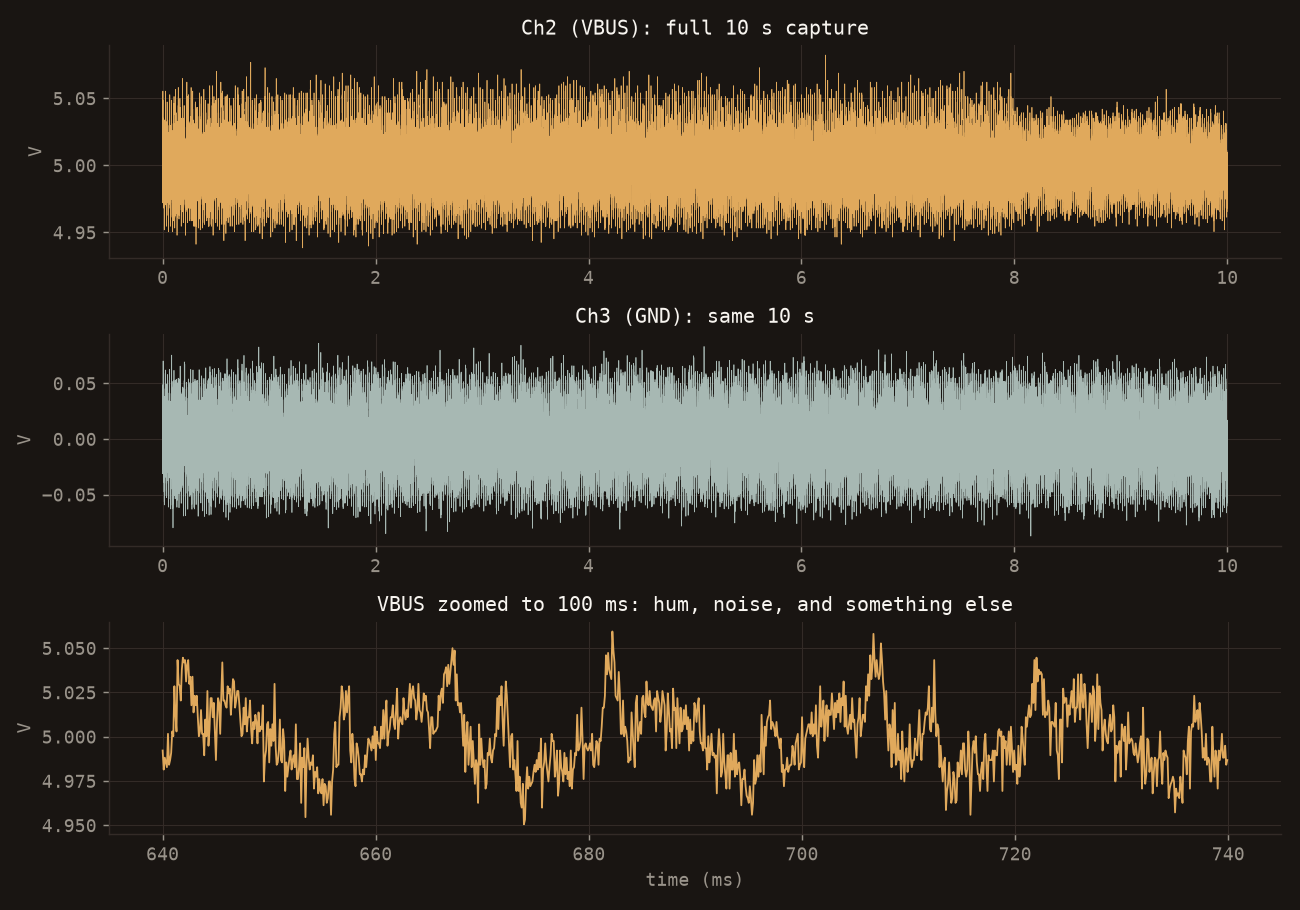
Ch2 and Ch3 over the whole capture, then VBUS zoomed to 100 ms
Over the full 10 s, both channels look like noise. Notice that the VBUS band gets thinner after the 8 s mark, where the transmission ends. Zoomed in, VBUS has a slow wave (the 50 Hz hum), random noise, and short spikes at a regular rhythm, about 30 mV tall on a 5 V rail.
Two more clues:
- VBUS and GND are correlated (r ≈ 0.55), because the hum is on both.
- The spikes repeat on a 10 ms grid.
Almost right isn’t a flag
A natural first attempt: for each 10 ms slot, find the most extreme sample and check which half of the slot it’s in. The challenge talks about “fluctuations”, and power problems are usually sags, so it’s tempting to reach for argmin:
def window_min_decode(signal):
    syms = []
    for i in range(len(signal) // SYM_N):
        win = signal[i * SYM_N: (i + 1) * SYM_N]
        syms.append(0 if np.argmin(win) < SYM_N // 2 else 1)
    return syms
It gets 136 of the 800 symbols wrong. The pulses point up, so the deepest point in each slot is one of the Ricker’s side lobes, which are only about 13 mV deep, and the noise wins often.
Once you notice that and switch to argmax, it looks solved: only 14 of 800 symbols wrong (98% right). Here is what that decodes to:
argmax, raw:      Securinets{u3b_p0w3r_l1n3\x1f3xf1ltr4u10~}      CRC ✗
argmax, cleaned:  Sec\xf5rinets{usb_p0w1r_l1n3_3xvqltr4t10n}      CRC ✗
Readable, and still wrong. You could probably guess the flag by combining the two, but a guess is still a guess, and the CRC says it’s wrong.
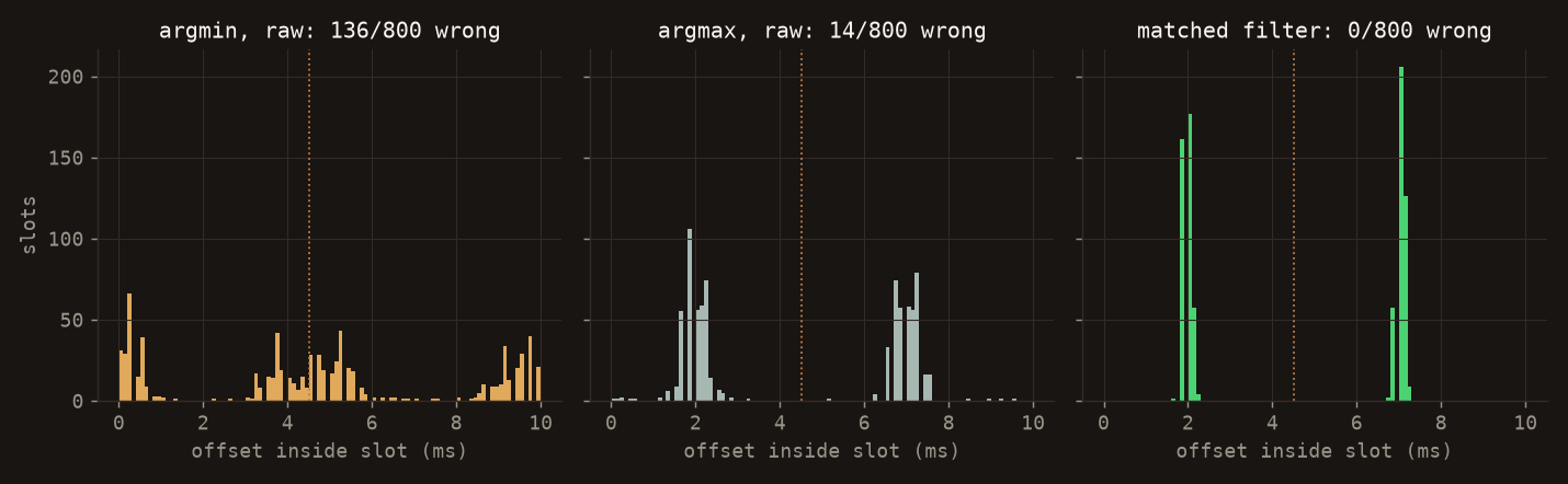
Where each method places the pulse inside its slot, over the 800 slots that carry data. The dotted line is the 4.5 ms decision boundary
The histograms show what’s going on:
argminspreads across the whole slot. Its clusters are the side lobes (around 0.3/3.7 ms and 5.3/8.7 ms), not the pulses.argmaxfinds the pulses, but the clusters are wide, and a few outliers land on the wrong side of the line.- The matched filter (below) puts every pulse in a tight spike at exactly 2 ms or 7 ms.
The underlying issue is that picking one sample is a weak decision. At 10 kS/s the pulse’s main lobe is about 20 samples wide, and a single-sample decision ignores 19 of them.
The fix: clean up, then correlate
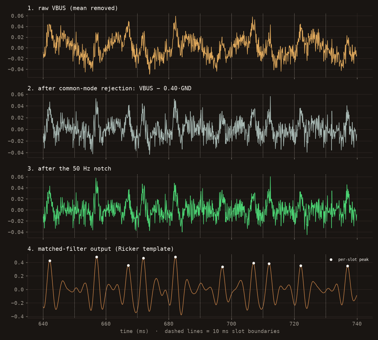
The same 100 ms window at each stage of processing
Step 1: common-mode rejection with GND. The hum is on both channels, so estimate how much of GND is in VBUS (least squares) and subtract it:
def apply_cmr(vbus, gnd):
    v = vbus.astype(np.float64); g = gnd.astype(np.float64)
    v -= np.mean(v); g -= np.mean(g)
    alpha = np.mean(v * g) / np.mean(g * g)   # ≈ 0.40 here
    return v - alpha * g
This is why the GND channel is in the capture: it’s the reference, the same idea as a differential probe.
There’s a subtle catch. VBUS really carries 0.6× the hum that’s on GND, but the estimate comes out at 0.40. GND carries its own noise, and least squares shrinks the estimate by hum power / (hum power + noise power). With a 30 mV hum and 15 mV of GND noise, that’s (0.03²/2) / (0.03²/2 + 0.015²) = 2/3, and 0.6 × 2/3 = 0.40. So about a third of the hum survives step 1.
Step 2: a 50 Hz notch. A narrow IIR notch (Q = 30, about 1.7 Hz wide) removes what’s left of the hum without touching the ~1 ms pulses:
def notch_50hz(signal):
    w0 = 2.0 * math.pi * 50 / A_SR
    alpha = math.sin(w0) / 60.0          # Q = 30
    b = np.array([1.0, -2.0 * math.cos(w0), 1.0])
    a = np.array([1.0 + alpha, -2.0 * math.cos(w0), 1.0 - alpha])
    ...
After these two steps you can see the pulses by eye (panel 3), but single samples are still noisy.
Step 3: matched filter. When you know the pulse shape, the best linear detector in white noise is to correlate the signal with that shape. That uses every sample of the pulse instead of one. Measure the pulse width from a zoomed plot (~1 ms), build the template, and correlate:
def make_ricker_template():
    half = int(3 * PULSE_TAU * A_SR)
    n = np.arange(-half, half + 1) / (PULSE_TAU * A_SR)
    h = (1 - n * n) * np.exp(-n * n / 2)
    return h - np.mean(h)

mf = np.correlate(signal - np.mean(signal), templ, mode='same')
peaks = [t0 + np.argmax(mf[t0:t0 + SYM_N]) for t0 in range(0, n_syms * SYM_N, SYM_N)]
Panel 4 shows one clean peak per slot. Compare each peak’s offset to 4.5 ms (exactly halfway between 2 and 7 ms), decode the Manchester pairs, find 0xEB90, and check the CRC:
window-min:
  FAILED
matched filter:
  Securinets{usb_p0w3r_l1n3_3xf1ltr4t10n}
kalman+MF:
  Securinets{usb_p0w3r_l1n3_3xf1ltr4t10n}
eb 90  Securinets{usb_p0w3r_l1n3_3xf1ltr4t10n}  a4
                                               └─ CRC-8/MAXIM, matches
Zero symbol errors out of 800.
An alternative: Kalman + matched filter. My solver has a second path. On the cleaned signal, a small 2-state Kalman filter (level and slope) tracks whatever slow baseline is left, and its normalised innovation, meaning the part the model didn’t predict, goes into the same matched filter. It works like an adaptive high-pass filter and also gets zero errors. TX doesn’t need it, but it helps when the interference isn’t a neat 50 Hz tone.
Takeaways
- Power is a channel. Two devices that share a rail share a wire, even with no data connection between them.
- Blocking the data lines isn’t isolation. Charge-only cables, data blockers and device policies all leave VBUS and GND connected.
- Know the pulse shape before you pick a detector. On the same capture,
argmingot 136 of 800 symbols wrong,argmaxgot 14, and a matched filter got 0. - Use the reference channel you’re given. GND in the capture is there to be subtracted.
- Trust the error checks. Manchester pairs and the CRC tell you when a decode is right. 98% of symbols right still isn’t a flag.
Thanks to everyone who played GCUP 2.0, and to Securinets and the IFT for hosting it. If you solved TX a different way, message me. I’d like to see it.
References
- P. Kocher, J. Jaffe, B. Jun, Differential Power Analysis, CRYPTO ‘99.
- Y. Su, D. Genkin, D. Ranasinghe, Y. Yarom, USB Snooping Made Easy: Crosstalk Leakage Attacks on USB Hubs, USENIX Security 2017.
- P. Cronin, X. Gao, C. Yang, H. Wang, Charger-Surfing: Exploiting a Power Line Side-Channel for Smartphone Information Leakage, USENIX Security 2021.
- M. Guri, B. Zadov, D. Bykhovsky, Y. Elovici, PowerHammer: Exfiltrating Data from Air-Gapped Computers through Power Lines, 2018.